
As interest in analytics continues to grow, both analytics and data science increasingly show up in the course of business discussions. One domain that analytics has impacted is the marketing department. For example, marketers often evaluate A/B tests to improve their marketing results.
For example, many marketing departments are now sophisticated in their use of experimentation. Techniques such as A/B testing allow marketers to perform an experiment on how to engage customers, and then adjust their methods accordingly. Moreover, technology and digital platforms make it easier to execute A/B tests.
However, the analytical techniques to evaluate A/B tests in marketing are still not widely known. Many marketers have the tools to perform A/B testing, but not necessarily the tools to make business decisions based on A/B tests. On the other hand, these analytical techniques have been available for decades. They are also used in other domains, such as biostatistics.
Thus, we should ask whether we can adopt the same techniques used in other domains to evaluate A/B tests for better marketing results.
The setup to evaluate A/B tests
Consider the following example. Suppose we run a marketing experiment involving two different promotional offers on two sets of customers, randomly selected:
- 625 offers in a test group
- 696 offers in the control group
After our marketing campaign ends, the results of the two promotional offers is as follows.
| Test (Group A) | Control (Group B) | |
|---|---|---|
| Accept | 32 | 14 |
| Decline | 593 | 682 |
Now, when we evaluate our results, we see that:
- Group A had 32 acceptances out of 625 offers, for a 5% response rate
- Group B had 14 acceptances out of 696 offers, for a 2% response rate
Can we conclude that our test was a success? If so, then we should adopt the new approach over the previous (control) approach to promotional offers.
However, before we make marketing changes, we want to calculate a confidence interval for our A/B tests. Formally, a confidence interval provides an estimated range for the odds ratio, if we repeatedly ran the experiment.
The analytics to evaluate A/B tests
To formalize the previous example, let’s define the variables n11 through n22 as follows.
| Test (Group A) | Control (Group B) | |
|---|---|---|
| Accept | n11 | n12 |
| Decline | n21 | n22 |
First, we define the odds ratio of an A/B test as the rate of the probability of a customer accepting offer A, relative to the probability of a customer accepting offer B.
Next, a confidence interval for the odds ratio is the probability that, if we ran the experiment repeatedly, the value of the odds ratio would fall somewhere in the interval.
Formally, we calculate the odds ratio as follows.
![]()
To calculate the confidence interval, we can use the delta method. So, we calculate:
- The standard error (SE) of the log odds ratio
- The log confidence interval (CIlog) from the log of the odds ratio and the standard error of the log odds ratio
- The confidence interval (CI) from the log confidence interval
The formulas are shown below:

Finally, we conclude that the test is successful if the range of the confidence interval does not include the value 1.
This all may sound complex, but it is mostly just straightforward math.
Example 1
So let’s get back to our prior example.
| Test (Group A) | Control (Group B) | |
|---|---|---|
| Accept | 32 | 14 |
| Decline | 593 | 682 |
Suppose that we want a 95% confidence interval. We can look up the appropriate value for Zα in a table for confidence intervals. The value is 1.96 for a 95% confidence interval.
When we run through the calculations:
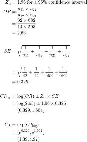
Thus, the odds ratio of our A/B test was 2.63. In other words, customers receiving the test offer were 2.63 times more likely to accept, compared to customers who received the control offer.
The 95% confidence for the confidence interval for the odds ratio ranges from 1.39 to 4.97. In other words, our test approach will be between 1.39 to 4.97 times more effective than our control approach, 95% of the time, if this test were to be repeated.
Since the value of 1 is not in our confidence interval, we would conclude that the test approach is superior to the control approach, and adjust our marketing efforts accordingly.
Example 2
Now, we can ask, “What happens when the value of 1 is in the confidence interval?” So, let’s consider another example.
Suppose that we run another A/B test and have the following test results.
| Test (Group A) | Control (Group B) | |
|---|---|---|
| Accept | 23 | 13 |
| Decline | 752 | 803 |
Again, suppose that we want a 95% confidence interval. When we run through the calculations:
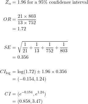
In this case, our odds ratio is 1.72. The 95% confidence interval for the odds ratio ranges from 0.858 to 3.47. So, it includes the value of 1.
In other words, our test approach will be between 0.858 to 3.47 times more effective than our control approach, 95% of the time, if this test were to be repeated. However, because 0.858 is less than 1, we cannot say with 95% confidence that the new method is better than our current method. Thus, it’s time for further experimentation in this example.
Lastly, for completeness, the python code for this example looks like this:
import numpy as np

z = 1.96 # for a 95% confidence interval
n11, n12, n21, n22 = 21, 13, 752, 803
odds = (n11*n22)/(n21*n12)
se = np.sqrt(1/n11 + 1/n12 + 1/n21 + 1/n22)
logCI = (np.log(odds) - z*se, np.log(odds) + 1.96*se)
CI = np.exp(logCI)
Personally, while I still find the theoretical basis behind the delta method challenging at times, the actual math and the code is not that bad.
Concluding thoughts on how to evaluate A/B tests
In conclusion, the delta method offers an elegant approach to provide statistical guarantees for a class of A/B tests, when we perform marketing experiments. It provides a more informed approach to evaluate A/B testing.
Now, in this article, we only covered binary A/B tests, where customers could either accept or decline a promotional offer. For other scenarios, such as evaluating A/B tests where values can range, such as total dollar spent, we can adopt other statistical techniques. For example, we can calculate lift and effect size to evaluate an A/B test in increasing total customer spend.
Second, a note on confidence intervals. In our examples, we calculated 95% confidence intervals, using a value of 1.96 for Zα. A 95% confidence interval is the standard for controlled experiments. Nonetheless, we could still consider a lower confidence interval.
For example, if we used an 80% confidence interval and a Zα value of 1.28, then the range for the confidence interval in Example 2 would, in fact, not contain 1. In other words, we would reject the test with a 95% confidence interval but would pass the test with an 80% confidence interval.






Two Ways To Calculate Sales Lift For Measuring Marketing Results
September 21, 2022[…] form of an odds ratio), but also a confidence interval for the sales lift. Coda Strategy also has additional examples of the odds ratio method with additional marketing […]